cl-random-forestでランダムフォレストの決定境界を描いてみる
cl-random-forestでは通常のランダムフォレストに加えて、ランダムフォレストの構造を使って特徴抽出し、それを線形分類器で再学習するという手法を実装している(Global refinement of random forest)。 通常のランダムフォレストに対して、この手法がどういう分類をしているかを見るために、二次元のデータでの実際の分類結果を可視化してみる。
このエントリではXORのデータで、綺麗に分かれている場合とかなりオーバーラップしている場合 とでランダムフォレストの決定境界を描いている。データはそれぞれのリンク先にある。
ランダムフォレストを構築
まずはXORのデータからランダムフォレストを構築する。完全なコードはここにある。
(defparameter *target*
  (make-array 100 :element-type 'fixnum
                 :initial-contents
                 '(1 1 0 1 1 0 1 0 1 1 0 0 1 0 0 0 1 0 0 0 0 0 1 1 0 1 1 1 0 0 0 1 1 1 1 1 1 1 0
                   0 1 1 0 0 1 0 0 1 0 1 1 1 1 1 1 0 1 0 1 1 0 0 0 0 1 0 0 1 1 1 1 0 1 0 0 1 0 1
                   0 0 0 0 0 1 0 1 0 1 1 0 0 1 0 0 1 0 0 1 1 0)))

(defparameter *datamatrix*
  (make-array '(100 2)
              :element-type 'double-float
              :initial-contents
              '((1.7128444910049438d0 -1.1600620746612549d0)
                (1.0938962697982788d0 -1.4356023073196411d0)
                (1.6034027338027954d0 0.6371392607688904d0)
                ...
                (-1.1475433111190796d0 0.9125188589096069d0)
                (0.5465568900108337d0 -0.3704013228416443d0)
                (1.1223702430725098d0 2.0434348583221436d0))))

;;; make random forest
(defparameter *forest*
  (make-forest *n-class* *n-dim* *datamatrix* *target* :n-tree 100 :bagging-ratio 1.0 :max-depth 100))

;;; test random forest
(test-forest *forest* *datamatrix* *target*)
; Accuracy: 100.0%, Correct: 100, Total: 100
可視化
プロットには以前実装したgnuplotのフロントエンドclgplotを使う。(解説記事)
splot-matrix関数でCommon Lispの二次元配列を三次元カラーマップでプロットすることができる。ここではmake-predict-matrixでプロット用の二次元配列を作っている。この関数には行列の一辺のサイズと定義域、さらに学習済みのモデルと訓練データを与える。
まずモデルから定義域全体の予測結果を出して、配列を埋めていく。次に配列中の各訓練データ点に相当する位置にラベルを表す1/-1を入れていく。
;;; plot decision boundary
(ql:quickload :clgplot)

(defun make-predict-matrix (n x0 xn y0 yn forest datamatrix target)
  (let ((x-span (/ (- xn x0) (1- n)))
        (y-span (/ (- yn y0) (1- n)))
        (mesh-predicted (make-array (list n n)))
        (tmp-datamatrix (make-array '(1 2) :element-type 'double-float)))
    ;; mark prediction
    (loop for i from 0 to (1- n)
          for x from x0 by x-span do
            (loop for j from 0 to (1- n)
                  for y from y0 by y-span do
                    (setf (aref tmp-datamatrix 0 0) x
                          (aref tmp-datamatrix 0 1) y)
                    (setf (aref mesh-predicted i j)
                          (if (> (predict-forest forest tmp-datamatrix 0) 0)
                              0.25 -0.25))))
    ;; mark datapoints
    (let* ((range (clgp:seq 0 (1- n)))
           (x-grid (mapcar (lambda (x) (+ (* x x-span) x0)) range))
           (y-grid (mapcar (lambda (y) (+ (* y y-span) y0)) range)))
      (loop for i from 0 to (1- (length target)) do
        (let ((data-i (position-if (lambda (x) (<= (aref datamatrix i 0) x)) x-grid))
              (data-j (position-if (lambda (y) (<= (aref datamatrix i 1) y)) y-grid)))
          (if (and data-i data-j)
              (setf (aref mesh-predicted data-i data-j)
                    (if (> (aref target i) 0) 1 -1))))))
    mesh-predicted))

(defparameter predict-matrix
  (make-predict-matrix 100 -3.5d0 3.5d0 -3.5d0 3.5d0 *forest* *datamatrix* *target*))

(clgp:splot-matrix predict-matrix)
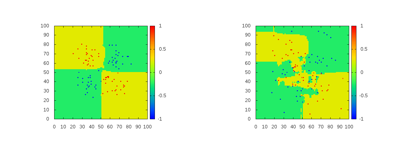
そうするとプロット結果は以下のようになる。
左が綺麗に分かれてるデータで右がオーバーラップしてるデータのときの分類結果を表している。どちらも訓練データを完璧に分類しているが、右の方ではあまりXORっぽくは見えない。特に、左上の外れ値に強く反応してかなりの領域を青側に誤判定してしまっている。
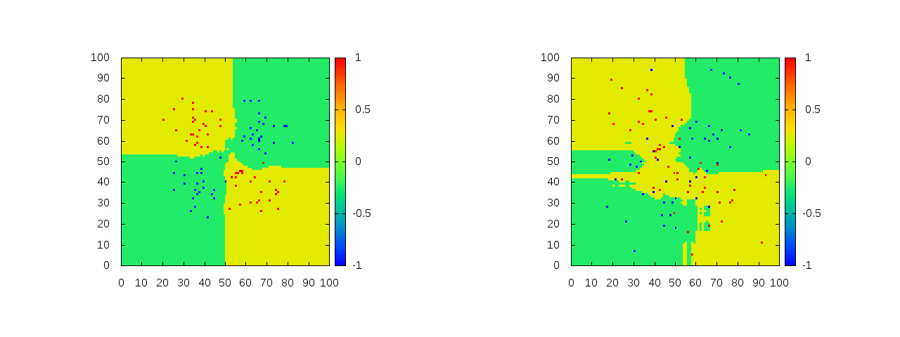
次の図は木の数を100から500にし、最大深さを100から15にし、バギング比率を1から0.1にしたときのもの。
上の図の条件下でさらにGlobal refinementを実行したもの。
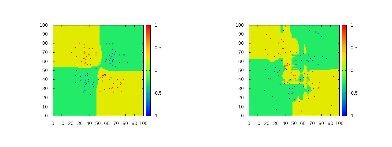
こうして見ると通常のランダムフォレストに対して外れ値に強くなり、より汎化性能が増しているよう見えなくもない。